Say hello to shadergarden

Hey, I'm Isaac Clayton, nice to meet you! This summer, I had the amazing opportunity to work as a software engineer intern at tonari, where I developed real-time stereo depth estimation algorithms for the GPU.

As I progressed further into my research, I was surprised by how slow some aspects of building a graphical pipeline were. To fill this gap, while working on implementing different algorithms, I also developed tooling to help remove some of the friction in the prototyping process.

At first, this tooling was just a jumble of utilities for hot-code reloading shaders. As time went on and I pruned, abstracted, and consolidated these utilities, I was pleasantly surprised when I saw a general tool for live-reloading shader pipelines emerge. We've initially called this tool shadergraph, for lack of a better name, but after some deliberation we've decided to release it as shadergarden, which I think is much more fun.

Today, we're excited to announce that we're open-sourcing shadergarden, a tool for developing shader-based graphical pipelines, under the MIT License. Source code, documentation, and the demos presented in this blog post are all in the repository up on GitHub.

Here are a few examples of what you can do with shadergarden:

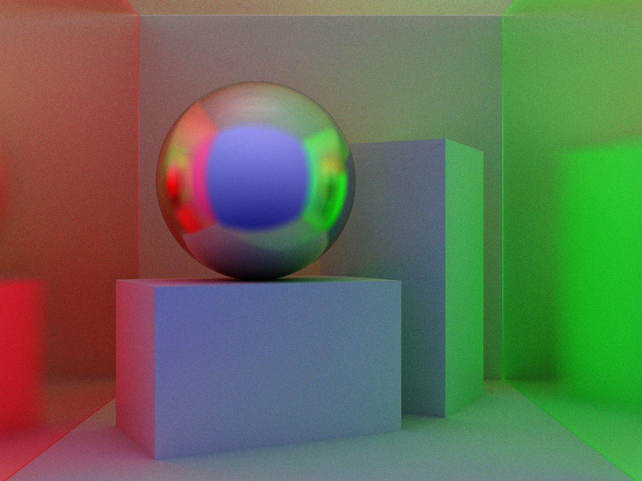
I deeply enjoy creating art with shaders, and I hope to share this passion with you. In this post, I hope to develop the rationale behind shadergarden and show you some pretty examples to pique your interest. So, let's talk about shaders.

Shaders!

What are shaders?

Traditionally, when we draw things on computers, we think like painters: draw a rectangle here, a triangle there, voilà! Under this model, we're looking at each shape and trying to figure out which pixels it colors.

Shaders are another way to draw things on computers. Unlike the above approach, they operate in an inverse manner: instead of calculating of which pixels a shape falls on, a shader calculates out which shapes fall on a pixel.

You can think of a shader as a function that returns a color given a point in 2D space. All shaders are provided with the same set of shared inputs, so the difference in color between pixels is a function of pixel alone.

There are a lot of crazy things that can be done with shaders. If you would like to learn how shaders work, I recommend reading The Book of Shaders and exploring the resources on Inigo Quilez's website.

It's best to have a loose intuition as to what shaders look like before we proceed, so here's an example shader that pulses through a slice of an RGB cube, the shader equivalent of a "Hello, World!"

// example.frag
// shadergarden flavored glsl
#version 140

in  vec2 coords;
out vec4 color;

uniform float u_time;

void main() {
    color = vec4(coords.xy, pow(sin(u_time), 2.), 1.);
}

The OpenGL Shading Language, or GLSL, is the most common shading language. Having a C-like syntax, the entry-point to all GLSL fragment shaders is the main function.

The primary way to pass inputs to shaders is through the use of uniforms. Uniforms can be many things, from numbers like floats to textures like sampler2D. In the above example, we have one uniform, u_time - it's conventional to use the u_ prefix to denote uniform values.

What about uniforms?

Uniforms are key to shadergarden, so it's best I explain them now. As mentioned earlier, a uniform is an input to a shader.

Uniforms are, well, uniform: they'll be the same across for every pixel in the shader. In other words, it's impossible to pass different uniforms to specific pixels. Instead, it's best to use something like a texture uniform, from which different values can be sampled depending on the coordinate of the pixel.

What's special about uniforms is that shaders produce textures, and textures can be uniforms; ergo, the output of one shader can be the input to the next. In this sense, we can chain shaders together, creating a series of passes to produce more complex outputs.

But chains aren't the only structure we're limited to. Because each shader can take multiple textures as input, we can build directed acyclic graphs of shaders, i.e. shader graphs, that can express arbitrarily complex graphical pipelines. Cultivating shader graphs live through hot-code reloading is a bit like growing a garden.

To describe these graphs in a reloadable manner, we need a language which is flexible enough to describe such graphs. We chose lisp to represent these pipelines, which we'll briefely discuss in the next section. The shadergarden Lisp Reference has more information about the specifics of the flavor of lisp we're using.

Getting started

Installation

If you have Rust installed, you can download shadergarden using Cargo:

cargo install shadergarden

You can also build from source if that's your thing. After installing shadergarden, check to see it's working by running shadergarden --version.

Let's make Conway's Game of Life!

Conway's Game of Life is a cellular automata that takes place on a 2D grid. Given an initial starting condition, each cell in the grid may change depending on its neighbors, so that the entire system evolves over time.

Each cell in Conway's game of Life is either dead or alive; each iteration, it may flip from one state to the other. To know whether a cell will be alive in the next iteration, we look at the 8 surrounding neighbor sells around a cell, and count how many of them are alive:

1. If the cell has 3 alive neighbors exactly, it will be alive in the next iteration.
2. If the cell only has 2 alive neighbors but is alive itself, it will be alive in the next iteration.
3. Otherwise, the cell will die or stay dead if it is already dead.

Because all cells are updated at the same time according to these rules, Life is easy to express using shaders, and is an ideal first project for getting started with shadergarden.

After you've verified shadergarden is installed, make a folder for this project - I've named mine life-graph - and add the following two files:

life-graph
├── life.frag
└── shader.graph

life.frag is a GLSL fragment shader, and shader.graph is our lispy configuration file describing the shader pipeline.

Let's start by setting up shader.graph. The driving loop behind Conway's Game of Life is relatively simple, so our graph is quite small:

(let life (shader-rec "life" 512 512))
(output life)

shader-rec is a simple keyword that defines a recurrent shader, meaning the output texture of the previous iteration becomes the input uniform of the next iteration. Here, shader-rec takes 3 arguments: the file stem of the shader, "life", tells shadergarden to load life.frag; the two numbers that follow 512 512, are the width and height out the output. We bind this recurrent shader to the variable life, and mark it as an output, i.e. the texture we want to display.

Now that the basic graph is defined, pop open life.frag. Let's get cracking!

// we're using an old version for compatibility
// but newer GLSL versions are supported as well
#version 140

uniform sampler2D u_previous;
uniform vec2      u_resolution;
uniform float     u_time;

#define PIXEL (1. / u_resolution)

in  vec2 coords;
out vec4 color;

// ...

First, we declare a number of uniforms, or inputs, to the shader. As this is a recurrent shader, we have access to the previous frame via the u_previous texture uniform. u_resolution is the width and height of the output texture; u_time is the time since the shader has started running. We also sneak in a definition for the width of a pixel relative to the size of the screen - this will come in handy later.

Remember, the code in shader is run over all pixels in parallel. Each pixel takes its normalized coordinate, coords, from 0 to 1, as input, and must produce an output color.

With the header out of the way, let's define an initial main entrypoint:

// ...

void main() {
    float alive = float(random(coords) > 0.5);
    color = vec4(vec3(alive), 1.);
}

Before we run any iterations of Conway's game of life, we need a starting condition. In the above code we just return a pseudorandom starting condition. There are lots of ways to define random numbers in GLSL, but the most common way by far is to truncate a high-frequency sine wave:

// from 'The Book of Shaders' chapter 10
float random(vec2 st) {
    return fract(sin(
        dot(st.xy,
            vec2(12.9898,78.233)))
        * 43758.5453123);
}

// ...

This gives us nice even random noise, which we then round to either 0 or 1:

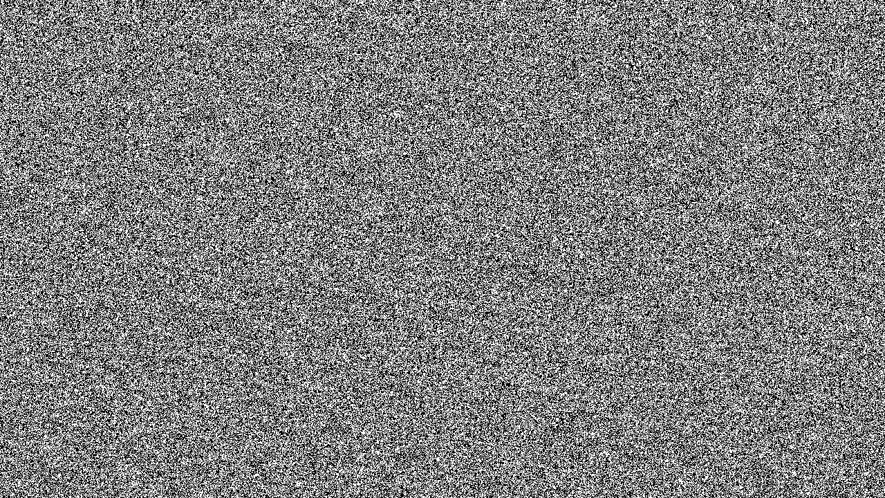
Great! Now that we have this basic shader defined, let's start shadergarden so we can take advantage of hot-code reloading and preview our changes live!

cd into life-graph (or whatever awesome name you've chosen), and run the following command:

shadergarden run

As soon as you hit enter, a new window should pop open and start running the graph.

shadergraph is now watching for changes, and will reload the graph on save. Keeping the running window open, slide over to life.frag — it's time to implement the rules of Life!

We'll start by defining a function called step_gol that calculates a single iteration of Life for a pixel. Here are the rules for Life as defined earlier:

1. If the cell has 3 neighbors exactly, it will be alive in the next iteration.
2. If the cell only has 2 neighbors but is alive itself, it will be alive in the next iteration.
3. Otherwise, the cell will die or stay dead.

These rules readily map to shader code:

// ...

float step_gol(vec2 st) {
    float neighbors = count_neighbors(st);

    if (neighbors == 3.
    || (neighbors == 2. && is_alive(st) == 1.)) {
        return 1.;
    }

    return 0.;
}

Perfect! We only have two functions left to define: is_alive, and count_neighbors. Let's start with is_alive, which is basically a texture lookup:

float is_alive(vec2 st) {
    st = mod(st, 1.);
    return texture(u_previous, st).r;
}

// ...

You may have noticed that we're setting st to mod(st, 1.). This causes the grid to wrap around at the edges, feigning infinite space. Using is_alive, let's define count_neighbors:

// ...

float count_neighbors(vec2 st) {
    float neighbors = 0. - is_alive(st);

    for (float i = -1.; i <= 1.; i++) {
        for (float j = -1.; j <= 1.; j++) {
            vec2 neighbor = vec2(
                st + i * PIXEL.x,
                st + j * PIXEL.y));
            neighbors += is_alive(neighbor);
        }
    }

    return neighbors;
}

This code looks at the surrounding 8 neighbors and counts how many are alive. As you can see, we subtract whether the current cell is alive, so that it does not influence the tally of its neighbors.

With everything needed for Life now implemented, all that's left is updating main to call step_gol each frame:

// ...

void main() {
    float alive = float(random(coords) > 0.5);

    // add the following lines:
    if (u_time > 0.1) {
        alive = step_gol(coords);
    }

    color = vec4(vec3(alive), 1.);
}

After you've added the above lines to your shader, hit save: the window should update instantly, and you should see a little world start playing out before you.

Congratulations! You can now say you've written a parallelized version of Conway's Game of Life that runs on the GPU! I encourage you to mess around with the code you've written, and share whatever you discover with others.

There are lots of cool directions your code can take from here. You can try changing the rule defined in step_gol, make it so that images can be used as a starting condition, or adding a colorized visualization layer. Only your imagination (and the power of your GPU, I guess), is the limit!

The above colorized image was rendered by adding a second accumulative pass to the graph. I'm not going to go into a lot of detail here; but in essence, we start by adding a new fragment shader to the project:

life-graph
├── life.frag
├── color.frag  # new!
└── shader.graph

This shader will take its previous output (u_previous) and the current Life iteration (u_texture_0), then produce a colorized result. In the above gif, color.frag copies over the current Life iteration, then decays each color channel at a different rate. This is one method, but there are a lot of other visualizations to be explored. After you've written a colorization shader, add the new node to your shader.graph:

(let life (shader-rec "life" 512 512))
(let color (shader-rec "life" 512 512 life))  ; new!
(output color)

That's it! I hope this short example shows how to get started with shadergarden, and compose multiple shaders together. If you'd like a detailed guide to shader composition, look no further than the shadergarden Lisp Reference.

Demos

To test the boundaries of shadergarden, we scheduled a few Shader Jams to explore what could be done with it. Here are a few of the experiments we did; all of these experiments can be found in the demos folder in the shadergarden repository, and can be run with:

shadergarden run path/to/demo

Curl Noise

Brian Schwind saw this paper on Curl Noise, a special type of incompressible procedural noise that resembles the eddies and vorticies formed by a fluid. There are a lot of cool effects that can be made using this noise, though the field it produces alone is pretty visually pleasing:

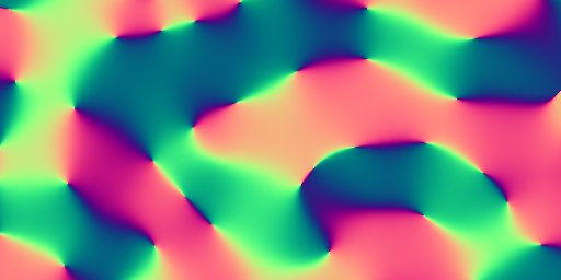
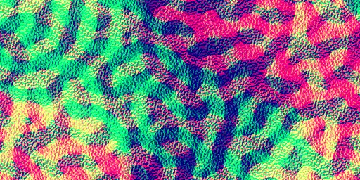
The second image is a stack of different-frequency curl noise added together, a la Fractional Brownian Motion.

Accumulative path tracer

There's a long tradition of rendering 3D scenes with shaders, so it's no surprise that I (Isaac Clayton) tried my hand at writing one. This is a Monte-Carlo path-tracing raymarcher, meaning ray distributions are probabilistically sampled and the scene is resolved by stepping through a signed distance field.

This initially results in noisy output; here's what we get out of the gate, after everything has been implemented:

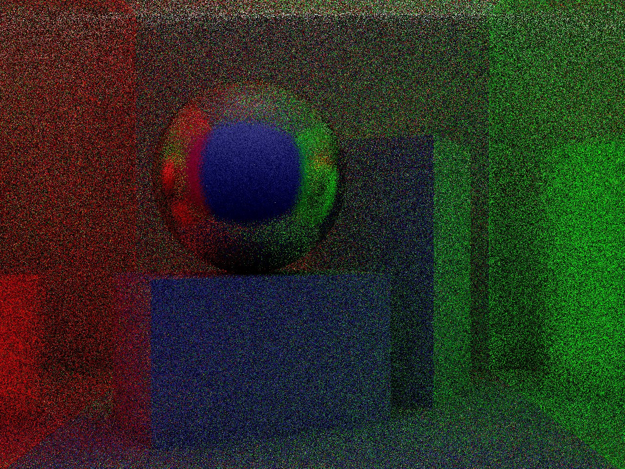
Although this video is pretty noisy, there are a few steps we can use to clean up the noise. The first is a accumulative filter, which averages successive frames; this cancels out noise over time. Starting from a black image, each added layer of samples further refines the image:

If the above video looks very dark, it's not just you. Because the accumulative average starts with a black frame, the brightness of the image will remain low until so many samples have been taken so that the initial black frame no longer holds any weight.

In a perfect world, we could take an infinite number of samples so this is no longer a problem. To approximate an infinite number of samples, we can brighten the progressive average by a constant determined by the number of samples taken so far. Doing this yields a brighter frame, which looks much better:

To clean up some remaining noise, I tried my hand at writing a denoising algorithm. The job of a denoiser is to smooth out regions of the image that should be, well, smooth, while still preserving sharp edges and other fine detail present in the image.

The results I got were mixed, but I figured I may as well include them anyway. The denoiser is simply many iterations of an edge-weighted 3⨯3 box blur; in essence, we try to average solid regions without spilling over the edges of objects. This produces good results with really low sample count, but as the sample count increases, the denoising becomes less necessary.

Note how flat regions, e.g. the faces of the cuboids, are very consistently colored. If you look at the sphere, you can see where denoising breaks down, inferring sharpness that the algorithm does not have enough information to resolve.

This entire pipeline, from start to finish, has 5 passes: sampling, averaging, brightening, edge-extraction, and denoising. Aside from one other graph used internally, this graph is probably the most complex ones I've written. I think this multi-pass monte-carlo path-tracing raymarcher with denoising - goodness, that's a mouthful - shows the flexibility of the pipelines one can create.

If you'd like to blow up your computer and run this rendering engine, here's the link to this shadergarden project.

Gravity Simulation

I've long thought about simulating gravitational waves using quantized fluid simulation methods. Although not physically correct, the basic idea is that each timestep, each unit mass emits a 'gravitational particle' in every direction. Using a method similar to Reintegration Tracking, we progressively update the simulated gravitational field.

Because this method is iterative, objects with high velocities can make gravitational waves. Here's a normalized visualization of the gravitational waves created by two objects orbiting each other at near the 'speed of light' (which in this universe is 1 pixel per frame).

This video was rendered at a resolution 512⨯512 with the speed of light set to 400 pixels per second; we adjusted the speed of the video a bit to make it more fun to watch. The source code for this demo can be found here, if you want to play around with it yourself.

Using shadergarden as a Rust library

Aside from using shadergarden as a CLI to live-prototype graphs of shaders, shadergarden was designed to be a library that easily integrates with other Rust projects. Currently, shadergarden supports glium as a backend, but in the (distant) future, we may add support for WGPU and other backends.

We understand that lisp may not be your jam: aside from shadergarden lisp, the library provides a number of methods for constructing graphs of shaders directly (which the lisp uses under-the-hood). If you're considering adding an extensible shader-based transformation pipeline to your project, why not give shadergarden a try?

Thank you!

I'm grateful I got the opportunity to intern at tonari this summer, and that I was able to publicly release some of the work I did. I especially appreciate the guidance and assistance my mentor Jake McGinty and my supervisor Ryo Kawaguchi provided, and would like to thank them sincerely. The rest of the tonari team is chock full of amazing people, and I'm glad I got to know everyone. If you're wondering what it's like to work as a remote intern at tonari, take a look at Edward Yang's post on the subject.

Get Creative!

Hey, thanks for reading this far! We've had a lot of fun working with shadergraph, and can't wait to see what y'all do with it. See you around!

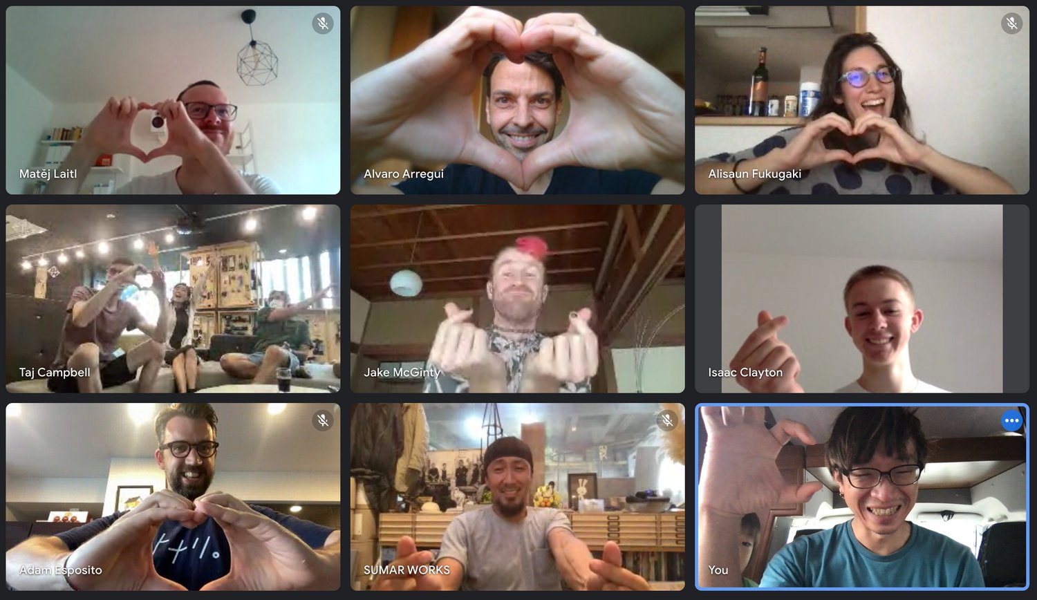
Thanks for reading! You can learn more about tonari and our team on our blog and website, and follow new developments via our monthly newsletter.

Find us 💙

Facebook: @heytonari Instagram: @heytonari X: @heytonari